First of all, give yourself a pat on the back! You’ve made it through parametric equations (9.1, 9.2, and 9.3) and vector-valued functions (9.4 and 9.5) and tied them together in solving motion problems in 9.6. Where do we go from there?

The last section of this unit deals with polar coordinates. In our introduction, they are briefly defined as part of a two-dimensional coordinate system dealing with a line’s distance from the origin (r) and the angle said line makes with the positive x-axis (θ)… but what does that really mean?

To understand polar coordinates, we need to understand the functions that utilize them the most: polar functions!

🐻‍❄️ What are Polar Functions?

Polar functions, also known as circular functions, are functions commonly graphed in a polar coordinate system, which uses a distance (r) from a fixed point, known as the pole, and an angle (θ) measured counter-clockwise from the positive x-axis, to determine the coordinates of a point. These functions are often used in physics and engineering to model phenomena such as waves, orbits, and fields. 🌊

Image courtesy of Math Insight

When working with polar functions, it can be difficult to differentiate them using traditional Calculus techniques because the functions are defined in terms of r and θ, rather than x and y.

To illustrate, take a look at the graphs below:

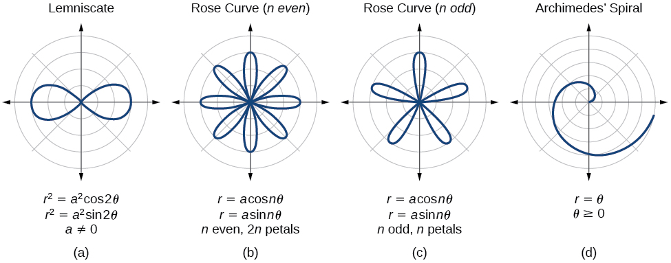
Image courtesy of Lumen Learning

Although they are aesthetically pleasing, it sounds like a nightmare to actually differentiate them when looking back to our definition of differentiation in the Cartesian plane—the slope of the tangent line at a point—as this doesn’t translate well in Polar-ville.

To overcome this limitation, we can convert polar equations to Cartesian equations by using the following relations:

x=rcos\theta\\y=rsin\theta

Converting polar equations to Cartesian equations also allows us to visualize the functions more easily, as they can be graphed on a traditional x-y coordinate plane. This can be especially useful when working with complex functions that have multiple parts, such as a combination of trigonometric and polynomial functions. 🦄

Another conversion to be mindful is the following:

r=\sqrt{x^2+y^2}

✏️ Converting Polar to Cartesian Practice

Let’s practice with some examples!

🥇 Converting Polar to Cartesian Example 1

Convert the following polar function to a Cartesian function:

r=4\sin\theta

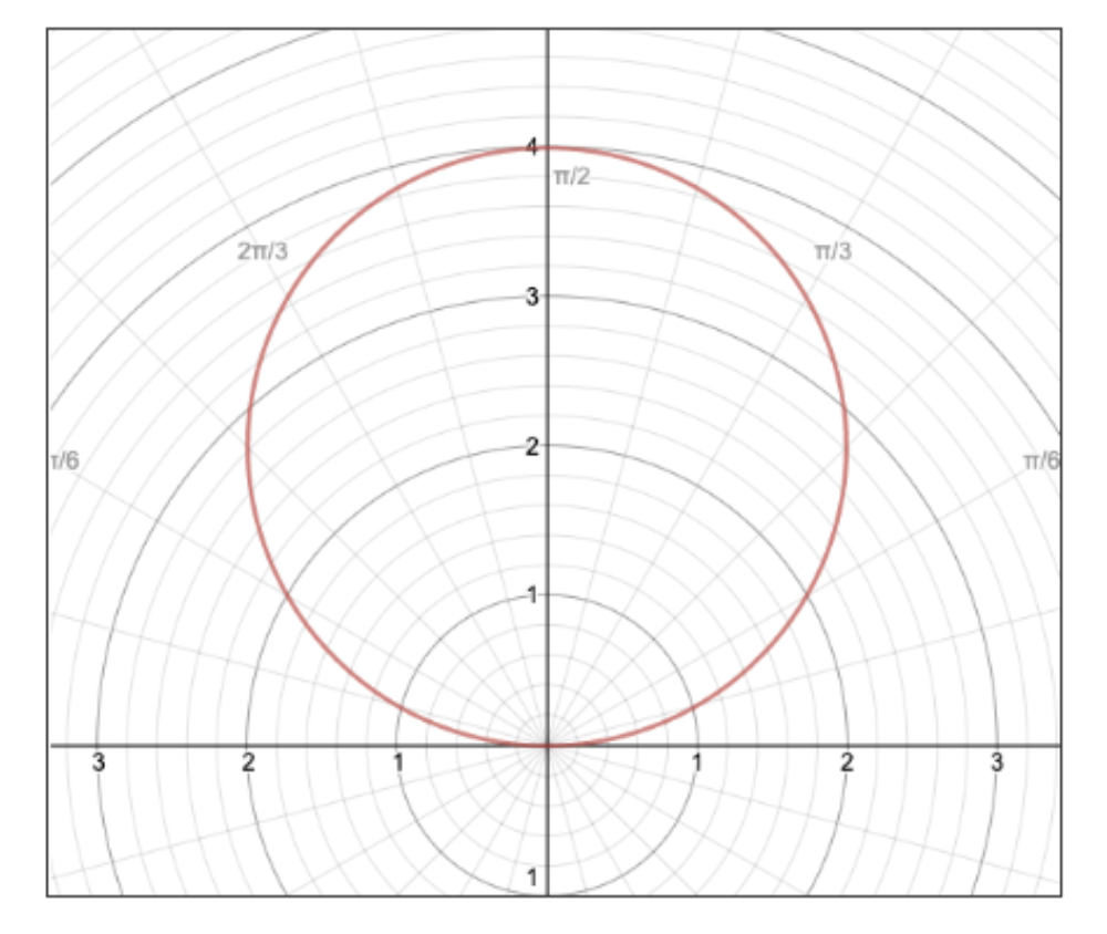
Image courtesy of Sumi Vora

To start, let’s rearrange our equation of interest:

\sin\theta=\frac{r}{4}

Aside, let’s bring out our best friend $y = r\sinθ$ , rearrange it, and set this equation equal to the above equation:

y=r\sin\theta=>\sin\theta = \frac{y}{r}=\frac{r}{4}\\r^2=4y

Now, we bring out our other best friend, the “square root” equation:

(\sqrt{x^2+y^2})^2=4y\\x^2+y^2=4y

Next, we do a bit of algebra magic (aka, completing the square) and get our final Cartesian function:

x^2+(y^2-4y)=0\\x^2+(y^2-4y+4)=4\\x^2+(y-2)^2=4

Ta-da! As you might’ve noticed, converting from polar to Cartesian (or vice versa) requires familiarity with the three essential equations above, relating x, y, r, and θ (with the help of sin). 🥳

Let’s change up the problem by adding values for x (or y)!

🥈 Converting Polar to Cartesian Example 2

Find the values of θ on $r = 2 + 3\sinθ$ where $x = 2$ .

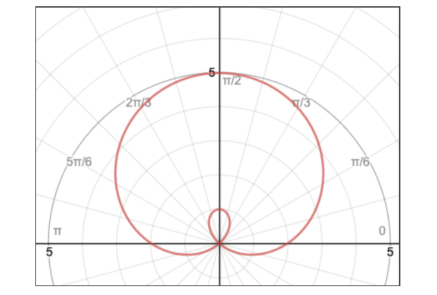
Image courtesy of Sumi Vora

We have two moving pieces here: the “r = …” and the “x = 2” equations. When you have these pieces, aim to connect the two in some way or form. In this case, we can plug in our x = rcosθ best friend into our x = 2 equality:

x=2\\r\cos\theta=2

As for the “r = …” equation, we can then plug this into what we got above:

r=2+3\sin\theta

(2+3\sin\theta)\cos\theta=2

2\cos\theta+3\sin\theta \cos\theta=2

Plugging this into your calculator (i.e., using a built-in solver function), you will get the following answers:

\theta=0\\\theta=1.133

Slightly more challenging, huh? The general principle, though, is still the same: you use what you know about our “best friend” equations to connect x, y, r, and θ. There is a pattern with these problems! 😁

💭Derivatives of Polar Functions

When we take derivatives of polar functions, we can take them as dr/dθ, which would give us the points that are furthest away from the origin on the polar coordinate system. We find dr/dθ in the same way we would find any normal derivative: by taking the derivative of the polar function. ⛰️

To illustrate, let’s work with an example!

✏️ Polar Function Derivative Walkthrough

Find the points closest and furthest from the origin for $r = θ + \cos(2θ)$ , $∈ [0, π)$ .

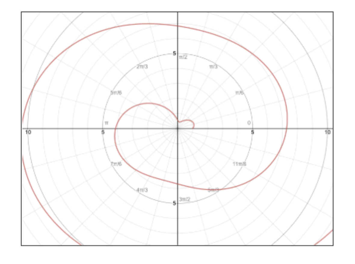
Image courtesy of Sumi Vora

We derive r with respect to θ, then set dr/dθ = 0 to solve for θ:

r=\theta+\cos(2\theta)\\\frac{dr}{d\theta}=1-\sin(2\theta)*2\\0=1-2\sin(2\theta)\\\frac{1}{2}=\sin(2\theta)

Thinking back to the unit circle in trigonometry, where does sin of something equal 1/2?

2\theta=\frac{\pi}{6},\frac{5\pi}{6}\\

\theta=\frac{\pi}{12},\frac{5\pi}{12}

Normally, we’d be done but wait! The question is asking for points, not angles. This means that we want the r values. We plug these angle values back into our original equation:

r(\frac{\pi}{12})=\frac{\pi}{12}+cos(2*\frac{\pi}{12})=1.128\\

r(\frac{5\pi}{12})=\frac{5\pi}{12}+cos(2*\frac{5\pi}{12})=0.443

Let’s do one last thing: check our endpoints, 0 and π, to see which one’s

r(0)=1\\r(\pi)=\pi

Our final answer? The point closest to the origin (0, 0) is 0.443, and the point furthest from the origin is π (3.141…). Relative to these points, 1 and 1.128 are in between close and far. That’s it! ✅

While dr/dθ can tell us relative maximum and minimum values, it doesn’t tell us the slope of the tangent line, since we can’t have linear graphs on the polar coordinate system. In order to find the slope of the tangent line, we need to find the derivative on the Cartesian system, which requires us to calculate dy/dx.

〰️ Slope of Tangent Line of Polar Functions

The one formula you need to know for this section:

\frac{dy}{dx}=\frac{dy/d\theta}{dx/d\theta}=\frac{\frac{d}{d\theta}(r\sin\theta)}{\frac{d}{d\theta}(r\cos\theta)}=\frac{r\cos\theta+\frac{dr}{d\theta}(\sin\theta)}{-r\sin\theta+\frac{dr}{d\theta}(\cos\theta)}

Of course, you can memorize this formula, but most students find it much easier to simply derive it using the chain rule.

✏️ Practice Finding Tangent Line to Polar Function

Find the equation of the line tangent to the polar curve $r = θ + \cos(2θ)$ at $θ = \fracπ3$ .

Yep, that’s the same polar function we saw in the last example! This time, we’re looking for dy/dx:

\frac{dy}{dx}=\frac{dy/d\theta}{dx/d\theta}\\

\frac{dy}{dx}=\frac{\frac{d}{d\theta}(\theta sin\theta+sin\theta cos2\theta)}{\frac{d}{d\theta}(\theta cos\theta+cos\theta cos2\theta)}=\frac{sin\theta+\theta cos\theta+cos\theta cos 2\theta-2sin\theta sin2\theta}{cos\theta-\theta sin\theta-sin\theta cos2\theta+2cos\theta sin 2\theta}

Substituting θ = π/3 into the equation:

\frac{sin\frac{\pi}{3}+\frac{\pi}{3} cos\frac{\pi}{3}+cos\frac{\pi}{3} cos 2\frac{\pi}{3}-2sin\frac{\pi}{3} sin2\frac{\pi}{3}}{cos\frac{\pi}{3}-\frac{\pi}{3} sin\frac{\pi}{3}-sin\frac{\pi}{3} cos2\frac{\pi}{3}+2cos\frac{\pi}{3} sin 2\frac{\pi}{3}}=0.429

Finding the x- and y-coordinates of the tangent line given what we know about r:

x=rcos\theta=(\frac{\pi}{3}+cos\frac{2\pi}{3})(cos\frac{\pi}{3})=0.274\\

y=rsin\theta=(\frac{\pi}{3}+cos\frac{2\pi}{3})(sin\frac{\pi}{3})=0.474

Therefore, the equation of the tangent line (in point-slope form) after putting everything together is:

y-0.474=0.429(x-0.274)

Still confused? Let's get into further detail:

When a curve is given by a polar equation, such as r = f(θ), it is represented in the polar coordinate system, where the position of a point is determined by its distance r from the origin and the angle θ that it makes with the positive x-axis. By taking the derivatives of the function r = f(θ) with respect to θ, we can learn important information about the curve, such as its curvature, concavity, and asymptotes.

🥇 The first derivative of r with respect to θ, denoted as r'(θ), is also known as the radial component of the curve, and it represents the instantaneous rate of change of the distance from the origin. It is also used to calculate the curvature of the curve, which is a measure of how sharply the curve bends at a given point.

🥈 The second derivative of r with respect to θ, denoted as r''(θ), is also known as the radial curvature of the curve, and it represents the rate of change of the curvature. It is also used to calculate the concavity of the curve, which is a measure of whether the curve is concave up or concave down at a given point.

In addition to derivatives of r, we can also find the x and y coordinates of a point on the curve in terms of θ by using the relations $x = r\cosθ$ and $y = r\sinθ$ . By taking the derivatives of x and y with respect to θ, we can learn important information about the tangent vector of the curve, and how it changes as we move along the curve.

Finally, by using the chain rule, we can find the first and second derivatives of y with respect to x. The first derivative is known as the slope of the curve, and it represents the rate of change of y with respect to x. The second derivative, again known as the curvature of the curve, represents the rate of change of the slope. 😁

🪐 Closing

…and that’s a wrap! Unlike parametric equations and vector-valued functions, polar coordinates are more finicky to work with because of the extra steps of converting between coordinate systems, applying trigonometric identities and remembering the unit circle, and oftentimes plugging into your calculator.

Even so, there is beauty in polar coordinates in a sense that we can find derivatives by applying relatively similar concepts from what we’ve learned earlier in the unit with parametric equations; only this time, we’re dealing with θ instead of t.

Like any other Unit 9 concept, practice, practice, practice until you can hit bullseyes one after another! 🎯

<< Hide Menu

📚

All Subjects

♾️

AP Calc

🦖

Unit 9

9.7 Defining Polar Coordinates and Differentiating in Polar Form

3 min read•june 18, 2024

Sumi Vora

Jed Quiaoit

Sumi Vora

Jed Quiaoit