Parametric equations
Polar coordinates - a two-dimensional coordinate system dealing with a line’s distance from the origin ( $r$ ) and the angle said line makes with the positive x-axis ( $θ$ ).
Vector-valued functions - functions that returns a vector after taking one or more variables.

We’ll dive deeper into the second and third topics in future sections; for now, we’ll focus on parametric functions as they actually tell us a lot of information about real-world phenomena like projectile and circular motion.

💭 What is a Parametric Function?

Parametric functions are a set of related functions where x and y are independent from each other, but they are connected using the dummy variable t, which represents time. When we use the Cartesian graph, we assume that we are moving along the x-axis in only one direction at a constant rate. However, parametric equations give us more freedom to manipulate horizontal motion. 🗺️

A parametric equation would look something like this:

x(t)=t^2-1, y(t)=3t

In this equation, your x-coordinate would be determined by $t² - 1$ and your y-coordinate would be determined by $3t$ . So, when t = 1, you would plot the point (0, 3). In a parametric equation, t isn’t actually on the graph; we just use t as our constant so that our points are independent from one another.

There are several methods for calculating derivatives of real-valued functions, such as the limit definition, the power rule, the product rule, and the quotient rule. These methods can be extended to parametric functions, which are functions that depend on both a real variable and one or more parameters.

One way to extend these methods to parametric functions is to treat the parameters as constants and use the usual rules for differentiation. For example, if a parametric function is given by $f(x,p) = px²$ , where x is the real variable and p is the parameter, then the derivative with respect to x can be calculated using the power rule as $df/dx = 2p*x$ .

However, our method for computing derivatives will actually be much simpler than the method above. Excited? 😄

✏️ Differentiating Parametric Equations

Like we discussed earlier, a parametric function is still graphed in 2D on an xy-plane, so if we wanted to find the slope of the tangent line, we would still need to find dy/dx. 🔍

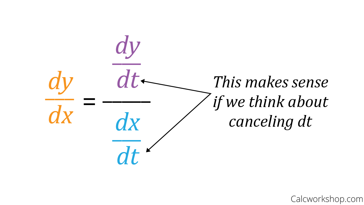
When dealing with parametric functions, where both x and y are expressed in terms of a third variable t, you can find the slope of the tangent line by taking the derivative of y with respect to t (dy/dt) and dividing it by the derivative of x with respect to t (dx/dt):

\frac{\frac{dy}{dt}}{\frac{dx}{dt}} = \frac{dy}{dx}

This ratio simplifies to dy/dx, which gives you the slope of the tangent line. This is analogous to the traditional approach of finding the slope of a curve in terms of x and y. Note than dx/dt cannot be zero!

🧠 Understanding Differentiation of Parametric Equations

Still confused about the theory? Let's go into further detail on what this idea really means physically and mathematically. 👇

This idea is known as the "parametric derivative" in calculus, often used to find the instantaneous rate of change of a parametric curve at a specific point. This method can only be used for parametric equations, where the curve is defined using a set of parametric equations in terms of a parameter, such as t.

To find the slope of the tangent line at a point on the curve, we first find the derivative of the x-coordinate function with respect to the parameter and the derivative of the y-coordinate function with respect to the parameter. These derivatives are denoted as dx/dt and dy/dt respectively. ⛰️

Then, at a specific point on the curve (x, y), the slope of the tangent line is found by taking the ratio of the derivative of the y-coordinate function with respect to the parameter (dy/dt) to the derivative of the x-coordinate function with respect to the parameter (dx/dt). This is the equation dy/dx = dy/dt / dx/dt we saw earlier! It’s important to note that the above equation is only valid if dx/dt is not equal to zero at the point of interest, as a vertical tangent line would not have a well-defined slope.

Now, this explanation still seems abstract when only talking about the theory. Why don’t we work this out with some examples? 😁

📝 Practice Differentiating Parametric Equations

Here are some concrete examples!

🥇 Differentiating Parametric Equations: Example 1

Find the slope of the tangent line of the parametrically defined equation at t = 3.

x(t)=t^2-2t, y(t)=t^2+1

We first need to find dy/dt (based on y(t)) and dx/dt (based on x(t)):

\frac{dx}{dt}=2t-2

\frac{dy}{dt}=2t

To get our final ratio dy/dx:

\frac{dy}{dx}=\frac{\frac{dy}{dt}}{\frac{dx}{dt}}=\frac{2t}{2t-2}=\frac{t}{t-1}

Normally, we’d stop here but we have a given parameter value (aka t = 3). Plug this into t:

\frac{dy}{dx}|_{t=3}=\frac{3}{3-1}=\frac{3}{2}

Therefore, the slope of the tangent line at t = 1 is $\frac32$ !

🥈 Differentiating Parametric Equations: Example 2

Find the slope of the tangent line of the parametrically defined equation at t = -1.

x(t)=ln(t), y(t)=3t^4+2t^5+3t-8

You know the drill: find dy/dt and dx/dt by deriving x(t) and y(t), respectively:

\frac{dx}{dt}=\frac{1}{t}

\frac{dy}{dt}=12t^3+10t^4+3

To get our final ratio dy/dx:

\frac{dy}{dx}=\frac{\frac{dy}{dt}}{\frac{dx}{dt}}=\frac{12t^3+10t^4+3}{\frac{1}{t}}=12t^4+10t^5+3t

Plug t = -1 into our result:

\frac{dy}{dx}|_{t=-1}=12(-1)^4+10(-1)^5+3(-1)=-1

Therefore, the slope of the tangent line at t = -1 is equal to -1!

💫 Closing

Feeling better? Like most of AP Calc, this unit becomes more and more navigable with practice and repeated exposure! It’s highly encouraged that you brush up on your derivatives and tangent line calculations from the differentiation-focused sections in earlier units. 🗒️

If you have limited time, the key takeaway for this section is the following:

As usual, good luck! 💯

Image Courtesy of CalcWorkshop.

<< Hide Menu

📚

All Subjects

>

♾️

AP Calc

>

🦖

Unit 9

9.1 Defining and Differentiating Parametric Equations

3 min read•june 18, 2024

Sumi Vora

Jed Quiaoit

Sumi Vora

Jed Quiaoit