Browse By Unit
1.13 Function Model Selection and Assumption Articulation
1 min read•june 18, 2024
1.13 Function Model Selection and Assumption Articulation
Now that we’ve explored rates of change, polynomial and rational functions, and even functions that transform, you might wonder: Where’s the IRL component? (In other words, “how do any of these apply to real life?”)
Well, you’re in luck! In this section, you’ll learn more about the logistics behind identifying an appropriate function type to construct a function model for a given scenario.
Function Models Based on Degree
In the context of functions in precalculus, a model is a mathematical representation of a real-world phenomenon or system. It’s a simplified representation of the system that is used to make predictions or understand the underlying relationships and processes. 🌎
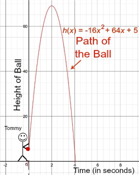
Source: Google Sites
Models can be represented using various types of functions, such as linear, quadratic, or exponential functions. These functions are chosen based on the characteristics of the system being modeled and the goals of the analysis. ☑️ Linear Functions****
Linear functions are often used to model data sets or aspects of contextual scenarios that demonstrate roughly constant rates of change. These functions have the general form of y = mx + b, where m is the slope and b is the y-intercept. Linear functions are useful for modeling systems where the rate of change is relatively constant, such as in direct variations or simple harmonic motion. 🫨
Example: A farmer wants to determine how much money he will make from selling his crops as a function of the number of acres he plants. He conducts an experiment and records the following data: 🧑🌾
- Number of acres planted (x): 0, 10, 20, 30, 40
- Money made from selling crops (y): 800, 2400, $3200
From this data, the farmer wants to create a linear model to predict how much money he will make for any given number of acres planted. To do this, he can use the equation of a line, y = mx + b, where m is the slope and b is the y-intercept.
To find the slope (m) and the y-intercept (b) of the model, the farmer can use the two points (0, 0) and (10, 800)
|
So, the linear model equation is y = 80x, which represents the linear relationship between number of acres planted and the money made.
Now he can use this equation to predict how much money he will make if he plants any number of acres. For example, if he plants 50 acres, he can substitute x = 50 into the equation to find y = 80(50) = $4,000. 💰 Quadratic Functions****
Quadratic functions, on the other hand, are often used to model data sets or aspects of contextual scenarios that demonstrate roughly linear rates of change, or data sets that are roughly symmetric with a unique maximum or minimum value. These functions have the general form of , where a, b, and c are constants. ☂️
Quadratic functions are useful for modeling systems where the rate of change is increasing or decreasing, such as in parabolic motion, or in data sets that have a distinct maximum or minimum point, such as in the case of a parabola.
Example: Not very numbers-focused, but there are many real-world situations that deal with quadratics and parabolas! Here’s a couple sample applications of quadratic modeling:
- The path of a projectile, such as a missile or a satellite in space, can be modeled using a quadratic function to represent the parabolic trajectory 🚀
- The height of a roller coaster at different points in time 🎢
- The strength of a parabolic antenna, such as the one used in wireless communication systems 📡
- In finance, the price of a stock over time can be modeled using a parabolic function to understand the trends in the stock market. 📈
- In physics, the motion of a simple pendulum can also be modeled by a quadratic function, which represents the parabolic path of the pendulum's bob.
- In engineering, the stress distribution in a parabolic arch
- In agriculture, the yield of a crop as a function of the amount of fertilizer applied
- In chemistry, the reaction rate of a chemical reaction can be modeled by a quadratic function, when the reactant concentrations are varied. 🧪
🔺 Context Clues: Geometry!
In geometric contexts, quadratic functions are often used to model two-dimensional shapes such as parabolas, ellipses, and hyperbolas. These shapes are often used to model systems involving area, such as in the case of geometric shapes like circles, ellipses, and parabolas. 🔵
Cubic functions, on the other hand, can be used to model three-dimensional shapes and systems involving volume, such as in the case of a sphere or a cube. These functions have the general form of , where a, b, c and d are constants. 🧊
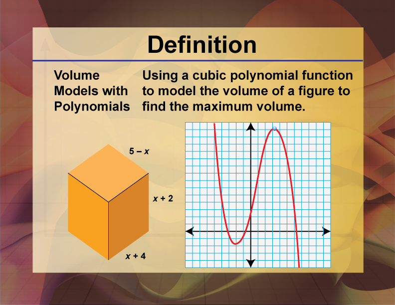
Source: Media4Math
Polynomial and Piecewise Functions
Polynomial functions are often used to model data sets or contextual scenarios with multiple real zeros or multiple maxima (high points) or minima (low points). In general, A polynomial function is a function of the form , where n is the degree of the polynomial, and are constants. 🚗
The degree of a polynomial function determines the highest power of x in the function.
A polynomial function of degree n models data sets or contextual scenarios that demonstrate roughly constant nonzero nth differences. This means that if you take the difference of the function's values at different inputs, and you keep taking differences, the resulting sequence will be roughly constant and nonzero if the function is of degree n.
A polynomial function of degree n or less can be used to model a graph of n + 1 points with distinct input values. This is because a polynomial function of degree n can be determined by n + 1 points. It means that if you have n+1 points, you can construct a polynomial function that passes through all of them. 🌈
Meanwhile, a piecewise-defined function is a function that is defined over different domains, and can be useful for modeling a data set or contextual scenario that demonstrates different characteristics over different intervals. 🧩
For example, a piecewise-defined function could be used to model a manufacturing process where the machine has different capabilities at different times of the day or week, or a function that models the behavior of a system that changes its behavior in response to certain inputs.
Piecewise-defined functions can be defined in many ways, but usually consist of different polynomials or other functions defined over nonoverlapping domain (x) intervals. They can also be defined using different equations or formulas for different intervals. This allows the function to model different behaviors over different intervals, making it a powerful tool for modeling complex systems.
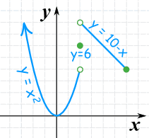
Source: Math is Fun
Assumptions and Restrictions
- Models may have underlying assumptions about what is consistent in the model. These assumptions may be based on mathematical clues or on contextual information about the system being modeled. For example, a model of a physical system may assume that certain laws of physics hold true, such as the conservation of energy. ⚡️
- A model may also have underlying assumptions about how quantities change together. For example, a model of the relationship between temperature and pressure may assume that these two quantities are directly proportional to each other. These assumptions are important because they allow the model to make predictions and understand the underlying relationships and processes. 🌡
- A model may also require domain restrictions based on mathematical clues, contextual clues, or extreme values in the data set. Domain restrictions are the values of the input variable (x) that are allowed in the function. For example, a model of the distance a projectile travels may be restricted to non-negative values of time, since it doesn't make sense to consider negative time in real-world scenarios.
- A model may also require range restrictions, such as rounding values, based on mathematical clues, contextual clues, or extreme values in the data set. Range restrictions are the values of the output variable (y) that are allowed in the function. For example, a model that predicts the cost of a product may only allow non-negative values, because it doesn't make sense to consider negative costs.
In the sample function below (y = 1/x), the restrictions are x and y can’t equal 0. (Otherwise, the function is undefined!)
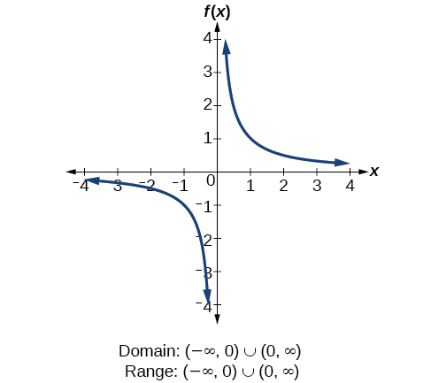
Source: Math LibreTexts
Keep in mind that models are not always perfect, and that they may not always represent the real-world system perfectly. Therefore, it's important to consider the underlying assumptions, domain and range restrictions, and the limitations of a model when interpreting its results and making predictions; even so, models are reliable in capturing the general trend behind a certain behavior or phenomenon observe in real life! 😁
<< Hide Menu
1.13 Function Model Selection and Assumption Articulation
1 min read•june 18, 2024
1.13 Function Model Selection and Assumption Articulation
Now that we’ve explored rates of change, polynomial and rational functions, and even functions that transform, you might wonder: Where’s the IRL component? (In other words, “how do any of these apply to real life?”)
Well, you’re in luck! In this section, you’ll learn more about the logistics behind identifying an appropriate function type to construct a function model for a given scenario.
Function Models Based on Degree
In the context of functions in precalculus, a model is a mathematical representation of a real-world phenomenon or system. It’s a simplified representation of the system that is used to make predictions or understand the underlying relationships and processes. 🌎

Source: Google Sites
Models can be represented using various types of functions, such as linear, quadratic, or exponential functions. These functions are chosen based on the characteristics of the system being modeled and the goals of the analysis. ☑️ Linear Functions****
Linear functions are often used to model data sets or aspects of contextual scenarios that demonstrate roughly constant rates of change. These functions have the general form of y = mx + b, where m is the slope and b is the y-intercept. Linear functions are useful for modeling systems where the rate of change is relatively constant, such as in direct variations or simple harmonic motion. 🫨
Example: A farmer wants to determine how much money he will make from selling his crops as a function of the number of acres he plants. He conducts an experiment and records the following data: 🧑🌾
- Number of acres planted (x): 0, 10, 20, 30, 40
- Money made from selling crops (y): 800, 2400, $3200
From this data, the farmer wants to create a linear model to predict how much money he will make for any given number of acres planted. To do this, he can use the equation of a line, y = mx + b, where m is the slope and b is the y-intercept.
To find the slope (m) and the y-intercept (b) of the model, the farmer can use the two points (0, 0) and (10, 800)
|
So, the linear model equation is y = 80x, which represents the linear relationship between number of acres planted and the money made.
Now he can use this equation to predict how much money he will make if he plants any number of acres. For example, if he plants 50 acres, he can substitute x = 50 into the equation to find y = 80(50) = $4,000. 💰 Quadratic Functions****
Quadratic functions, on the other hand, are often used to model data sets or aspects of contextual scenarios that demonstrate roughly linear rates of change, or data sets that are roughly symmetric with a unique maximum or minimum value. These functions have the general form of , where a, b, and c are constants. ☂️
Quadratic functions are useful for modeling systems where the rate of change is increasing or decreasing, such as in parabolic motion, or in data sets that have a distinct maximum or minimum point, such as in the case of a parabola.
Example: Not very numbers-focused, but there are many real-world situations that deal with quadratics and parabolas! Here’s a couple sample applications of quadratic modeling:
- The path of a projectile, such as a missile or a satellite in space, can be modeled using a quadratic function to represent the parabolic trajectory 🚀
- The height of a roller coaster at different points in time 🎢
- The strength of a parabolic antenna, such as the one used in wireless communication systems 📡
- In finance, the price of a stock over time can be modeled using a parabolic function to understand the trends in the stock market. 📈
- In physics, the motion of a simple pendulum can also be modeled by a quadratic function, which represents the parabolic path of the pendulum's bob.
- In engineering, the stress distribution in a parabolic arch
- In agriculture, the yield of a crop as a function of the amount of fertilizer applied
- In chemistry, the reaction rate of a chemical reaction can be modeled by a quadratic function, when the reactant concentrations are varied. 🧪
🔺 Context Clues: Geometry!
In geometric contexts, quadratic functions are often used to model two-dimensional shapes such as parabolas, ellipses, and hyperbolas. These shapes are often used to model systems involving area, such as in the case of geometric shapes like circles, ellipses, and parabolas. 🔵
Cubic functions, on the other hand, can be used to model three-dimensional shapes and systems involving volume, such as in the case of a sphere or a cube. These functions have the general form of , where a, b, c and d are constants. 🧊

Source: Media4Math
Polynomial and Piecewise Functions
Polynomial functions are often used to model data sets or contextual scenarios with multiple real zeros or multiple maxima (high points) or minima (low points). In general, A polynomial function is a function of the form , where n is the degree of the polynomial, and are constants. 🚗
The degree of a polynomial function determines the highest power of x in the function.
A polynomial function of degree n models data sets or contextual scenarios that demonstrate roughly constant nonzero nth differences. This means that if you take the difference of the function's values at different inputs, and you keep taking differences, the resulting sequence will be roughly constant and nonzero if the function is of degree n.
A polynomial function of degree n or less can be used to model a graph of n + 1 points with distinct input values. This is because a polynomial function of degree n can be determined by n + 1 points. It means that if you have n+1 points, you can construct a polynomial function that passes through all of them. 🌈
Meanwhile, a piecewise-defined function is a function that is defined over different domains, and can be useful for modeling a data set or contextual scenario that demonstrates different characteristics over different intervals. 🧩
For example, a piecewise-defined function could be used to model a manufacturing process where the machine has different capabilities at different times of the day or week, or a function that models the behavior of a system that changes its behavior in response to certain inputs.
Piecewise-defined functions can be defined in many ways, but usually consist of different polynomials or other functions defined over nonoverlapping domain (x) intervals. They can also be defined using different equations or formulas for different intervals. This allows the function to model different behaviors over different intervals, making it a powerful tool for modeling complex systems.

Source: Math is Fun
Assumptions and Restrictions
- Models may have underlying assumptions about what is consistent in the model. These assumptions may be based on mathematical clues or on contextual information about the system being modeled. For example, a model of a physical system may assume that certain laws of physics hold true, such as the conservation of energy. ⚡️
- A model may also have underlying assumptions about how quantities change together. For example, a model of the relationship between temperature and pressure may assume that these two quantities are directly proportional to each other. These assumptions are important because they allow the model to make predictions and understand the underlying relationships and processes. 🌡
- A model may also require domain restrictions based on mathematical clues, contextual clues, or extreme values in the data set. Domain restrictions are the values of the input variable (x) that are allowed in the function. For example, a model of the distance a projectile travels may be restricted to non-negative values of time, since it doesn't make sense to consider negative time in real-world scenarios.
- A model may also require range restrictions, such as rounding values, based on mathematical clues, contextual clues, or extreme values in the data set. Range restrictions are the values of the output variable (y) that are allowed in the function. For example, a model that predicts the cost of a product may only allow non-negative values, because it doesn't make sense to consider negative costs.
In the sample function below (y = 1/x), the restrictions are x and y can’t equal 0. (Otherwise, the function is undefined!)

Source: Math LibreTexts
Keep in mind that models are not always perfect, and that they may not always represent the real-world system perfectly. Therefore, it's important to consider the underlying assumptions, domain and range restrictions, and the limitations of a model when interpreting its results and making predictions; even so, models are reliable in capturing the general trend behind a certain behavior or phenomenon observe in real life! 😁

© 2024 Fiveable Inc. All rights reserved.