Browse By Unit
Jacob Jeffries
Jacob Jeffries
7.3 Sketching Slope Fields
Slope fields allow us to visualize a solution to a differential equation without actually solving the differential equation. Let’s construct a slope field to solidify this idea. 🧠
Slope fields essentially draw the slopes of line segments that go through certain points.
Example 1
Let’s consider the following differential equation:
The slope (m) at point (x,y), in this case, is just x + y, which we can put into a table for various coordinates:
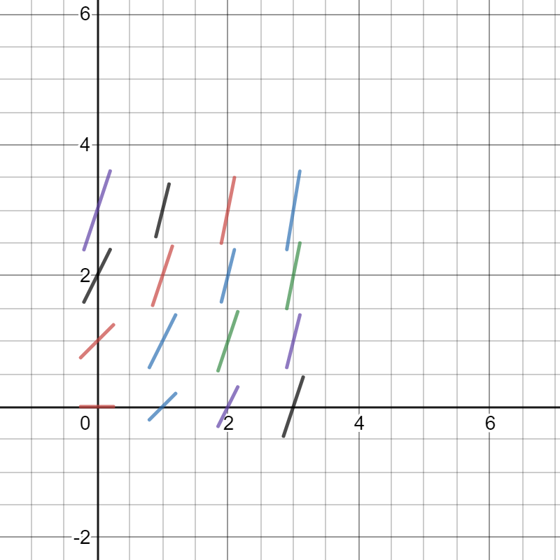
We can use this data to draw an approximate solution to the differential equation by drawing short line segments through each point that have the corresponding slope:

Source: Jacob Jeffries
Example 2
Let’s consider another differential equation:
The slope (m) at point (x,y), in this case, is just , which we can put into a table for various coordinates:
| undefined | ||||
| undefined | ||||
| undefined | ||||
| undefined |
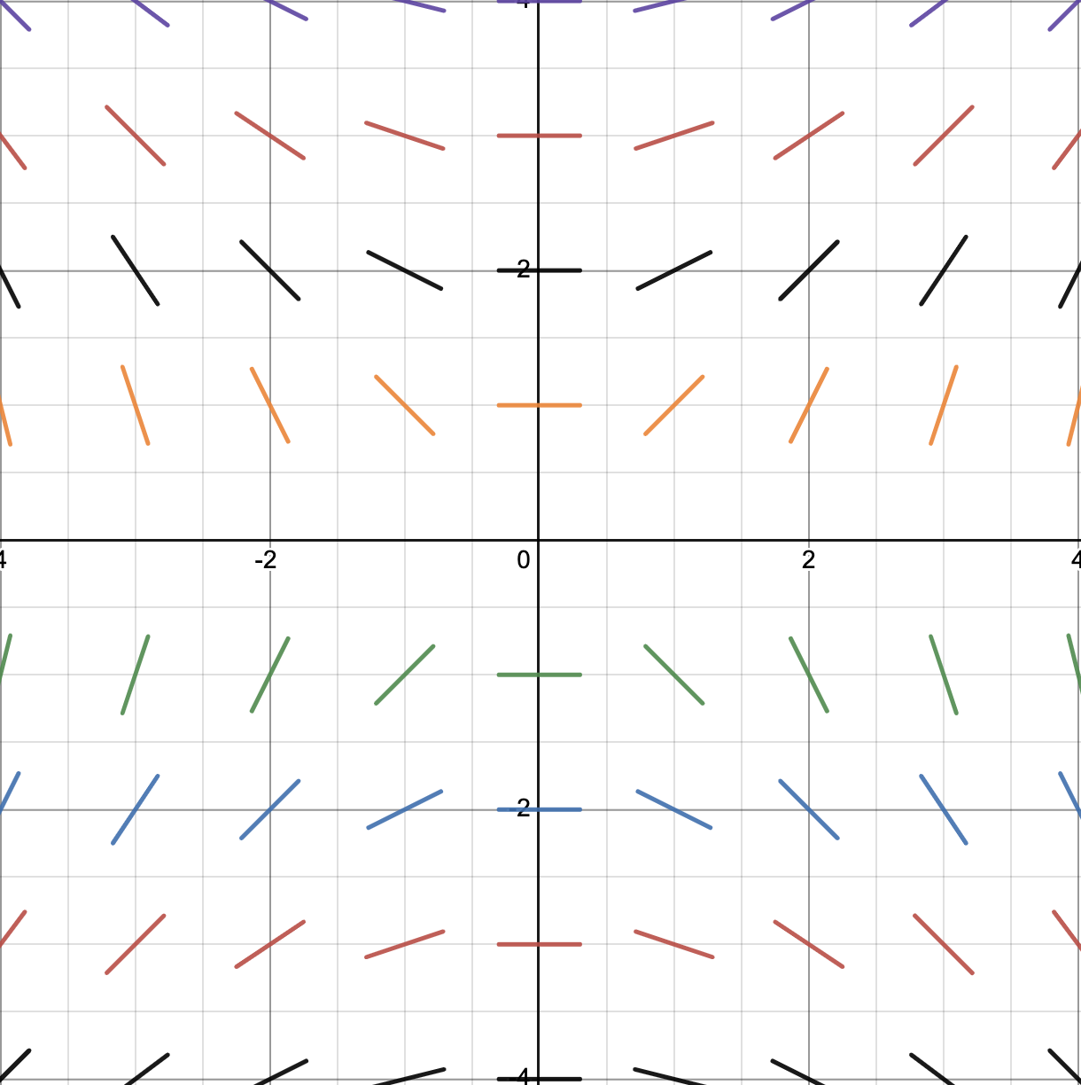
We can use this data to draw an approximate solution to the differential equation by drawing short line segments through each point that have the corresponding slope.
The graph below includes more points than in the table to provide you with a better illustration of what a slope field looks like:

Source: Jacob Jeffries
To be continued in 7.4 Reasoning Using Slope Fields.
<< Hide Menu
Jacob Jeffries
Jacob Jeffries
7.3 Sketching Slope Fields
Slope fields allow us to visualize a solution to a differential equation without actually solving the differential equation. Let’s construct a slope field to solidify this idea. 🧠
Slope fields essentially draw the slopes of line segments that go through certain points.
Example 1
Let’s consider the following differential equation:
The slope (m) at point (x,y), in this case, is just x + y, which we can put into a table for various coordinates:
We can use this data to draw an approximate solution to the differential equation by drawing short line segments through each point that have the corresponding slope:

Source: Jacob Jeffries
Example 2
Let’s consider another differential equation:
The slope (m) at point (x,y), in this case, is just , which we can put into a table for various coordinates:
| undefined | ||||
| undefined | ||||
| undefined | ||||
| undefined |
We can use this data to draw an approximate solution to the differential equation by drawing short line segments through each point that have the corresponding slope.
The graph below includes more points than in the table to provide you with a better illustration of what a slope field looks like:

Source: Jacob Jeffries
To be continued in 7.4 Reasoning Using Slope Fields.

© 2024 Fiveable Inc. All rights reserved.