Browse By Unit
Avanish Gupta
Jed Quiaoit
Avanish Gupta
Jed Quiaoit
When evaluating the effectiveness of a linear regression model, we use residuals to do this.
What is a residual, then?
Residuals are a measure of how well a linear regression model fits the data. They are the differences between the observed values of the response variable (y) and the predicted values (ŷ) from the model, so y - ŷ.
In a linear regression model, the goal is to find the line of best fit that minimizes the sum of the squared residuals. This is known as the least squares criterion. The residuals for each point represent the vertical distance between the point and the line of best fit. If a point has a small residual, it means that the model is predicting the value of the response variable well for that point. On the other hand, if a point has a large residual, it means that the model is not predicting the value of the response variable well for that point.
Here's another way to think about it, this time in terms of having "positive" and "negative" residuals: if we have a positive residual, then the actual value is greater than the predicted value and we say that the model underestimates the true value by a certain amount. Likewise, if we have a negative residual, then the actual value is less than the predicted value and we say that the model overestimates the true value by a certain amount.
Residual Plots
A residual plot is a graph that plots the residuals (the differences between the observed values and the predicted values) on the vertical axis and the predictor or explanatory variable on the horizontal axis. I
If the residual plot for a linear regression model exhibits apparent randomness, it can be taken as evidence that the relationship between the predictor and response variables is linear. In other words, it suggests that the model is capturing the underlying relationship in the data correctly.
"Apparent randomness" means that the residuals are randomly dispersed around the horizontal axis, as it indicates that the model is fitting the data well and that the residuals are not systematically related to the predictor variable.
Here are two examples of scatterplots with linear regression models (and also their residual plots).
Example 1
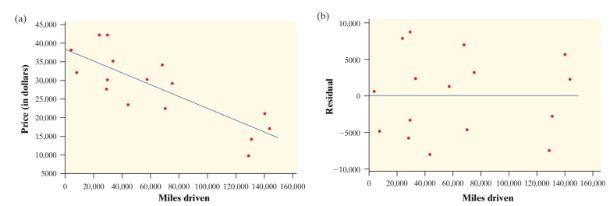
In the example below, we can see that our linear regression model fits our data fairly well (scatterplot on left). Therefore, the residual plot (on right) seems to show no apparent pattern. Our red points seem equally scattered about the red line at 0.
Courtesy of Starnes, Daren S. and Tabor, Josh. The Practice of Statistics—For the AP Exam, 5th Edition. Cengage Publishing.
Example 2
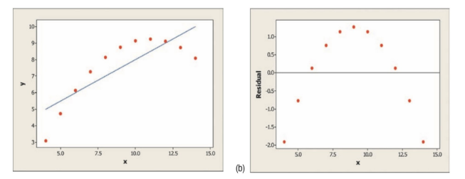
In this data, we can clearly see that our data follows a curved pattern, not the linear model pictured (scatterplot on left). Therefore, our residual plot (on right) shows an apparent curved pattern. We will learn more about these types of models in Unit 2.9 and how to adjust these to create a linear model.
Courtesy of Starnes, Daren S. and Tabor, Josh. The Practice of Statistics—For the AP Exam, 5th Edition. Cengage Publishing.
Good or Bad? 🧐
How do we tell whether a model is good? Look at the residual plot. For a good model, the residuals should be randomly scattered and have no clear pattern like with the first set above. In the second set, there is a distinct curve in the residual plot, meaning that a linear regression model is not appropriate to the scatterplot and a nonlinear model would be best.
Calculating Residuals
In order to calculate a residual for a given data point, we need the LSRL for that data set and the given data point.
We will first calculate the predicted value using the LSRL. Then, we subtract the predicted value from the actual value in the given data point. In other words, our formula is Residual = (Actual)-(Predicted).
Example 1
A LSRL model for the predicted amount of Lucky Charms eaten in accordance with one's age in years is given by the equation below:
ŷ=150.5x-2.34
A 50 year old from our data set is said to have eaten 7,500 lucky charms in his life! Wow! I hope he found the 💰 at the end of the 🌈! Calculate the residual for his number.
ŷ = 150.5(50) - 2.34
ŷ = 7522.66
Residual is 7500 - 7522.66= -22.66.
Keep in mind that sometimes you may be asked to calculate one's actual data point (or predicted data point) when given the residual. This would require the same formula, but working backwards.
Example 2
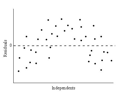
A researcher is studying the relationship between the number of hours spent studying for an exam and the score received on the exam. She collects data from 50 students and fits a linear regression model to the data. The residual plot for the model is shown below:
a) Describe the pattern, if any, in the residual plot.
b) Explain what the pattern in the residual plot suggests about the fit of the model.
c) If the model is not fitting the data well, suggest one potential reason why this may be the case.
d) Assuming that the model is not fitting the data well, propose one potential solution to improve the fit of the model.
e) Explain how the solution you proposed in part (d) would address the issue with the model.
Answers
a) The residual plot exhibits a curved pattern.
b) The pattern in the residual plot suggests that the fit of the model is not good. The residuals are not randomly dispersed around the horizontal axis, indicating that there is a systematic relationship between the predictor and response variables that is not being captured by the model.
c) One potential reason why the model may not be fitting the data well is that the relationship between the number of hours spent studying and the exam score is not linear. There may be some other underlying relationship between the variables that is not being captured by the model.
We'll learn more about d) and e) in future sections!
d) One potential solution to improve the fit of the model would be to transform the data in some way, such as by taking the logarithm of the number of hours spent studying or the exam score.
e) The solution proposed in part (d) would address the issue with the model by allowing the relationship between the predictor and response variables to be more accurately captured. A transformation may be able to uncover a more appropriate functional form for the relationship between the variables, leading to a better fit of the model.
🎥Watch: AP Stats - Least Squares Regression Lines
<< Hide Menu
Avanish Gupta
Jed Quiaoit
Avanish Gupta
Jed Quiaoit
When evaluating the effectiveness of a linear regression model, we use residuals to do this.
What is a residual, then?
Residuals are a measure of how well a linear regression model fits the data. They are the differences between the observed values of the response variable (y) and the predicted values (ŷ) from the model, so y - ŷ.
In a linear regression model, the goal is to find the line of best fit that minimizes the sum of the squared residuals. This is known as the least squares criterion. The residuals for each point represent the vertical distance between the point and the line of best fit. If a point has a small residual, it means that the model is predicting the value of the response variable well for that point. On the other hand, if a point has a large residual, it means that the model is not predicting the value of the response variable well for that point.
Here's another way to think about it, this time in terms of having "positive" and "negative" residuals: if we have a positive residual, then the actual value is greater than the predicted value and we say that the model underestimates the true value by a certain amount. Likewise, if we have a negative residual, then the actual value is less than the predicted value and we say that the model overestimates the true value by a certain amount.
Residual Plots
A residual plot is a graph that plots the residuals (the differences between the observed values and the predicted values) on the vertical axis and the predictor or explanatory variable on the horizontal axis. I
If the residual plot for a linear regression model exhibits apparent randomness, it can be taken as evidence that the relationship between the predictor and response variables is linear. In other words, it suggests that the model is capturing the underlying relationship in the data correctly.
"Apparent randomness" means that the residuals are randomly dispersed around the horizontal axis, as it indicates that the model is fitting the data well and that the residuals are not systematically related to the predictor variable.
Here are two examples of scatterplots with linear regression models (and also their residual plots).
Example 1
In the example below, we can see that our linear regression model fits our data fairly well (scatterplot on left). Therefore, the residual plot (on right) seems to show no apparent pattern. Our red points seem equally scattered about the red line at 0.

Courtesy of Starnes, Daren S. and Tabor, Josh. The Practice of Statistics—For the AP Exam, 5th Edition. Cengage Publishing.
Example 2
In this data, we can clearly see that our data follows a curved pattern, not the linear model pictured (scatterplot on left). Therefore, our residual plot (on right) shows an apparent curved pattern. We will learn more about these types of models in Unit 2.9 and how to adjust these to create a linear model.

Courtesy of Starnes, Daren S. and Tabor, Josh. The Practice of Statistics—For the AP Exam, 5th Edition. Cengage Publishing.
Good or Bad? 🧐
How do we tell whether a model is good? Look at the residual plot. For a good model, the residuals should be randomly scattered and have no clear pattern like with the first set above. In the second set, there is a distinct curve in the residual plot, meaning that a linear regression model is not appropriate to the scatterplot and a nonlinear model would be best.
Calculating Residuals
In order to calculate a residual for a given data point, we need the LSRL for that data set and the given data point.
We will first calculate the predicted value using the LSRL. Then, we subtract the predicted value from the actual value in the given data point. In other words, our formula is Residual = (Actual)-(Predicted).
Example 1
A LSRL model for the predicted amount of Lucky Charms eaten in accordance with one's age in years is given by the equation below:
ŷ=150.5x-2.34
A 50 year old from our data set is said to have eaten 7,500 lucky charms in his life! Wow! I hope he found the 💰 at the end of the 🌈! Calculate the residual for his number.
ŷ = 150.5(50) - 2.34
ŷ = 7522.66
Residual is 7500 - 7522.66= -22.66.
Keep in mind that sometimes you may be asked to calculate one's actual data point (or predicted data point) when given the residual. This would require the same formula, but working backwards.
Example 2
A researcher is studying the relationship between the number of hours spent studying for an exam and the score received on the exam. She collects data from 50 students and fits a linear regression model to the data. The residual plot for the model is shown below:

a) Describe the pattern, if any, in the residual plot.
b) Explain what the pattern in the residual plot suggests about the fit of the model.
c) If the model is not fitting the data well, suggest one potential reason why this may be the case.
d) Assuming that the model is not fitting the data well, propose one potential solution to improve the fit of the model.
e) Explain how the solution you proposed in part (d) would address the issue with the model.
Answers
a) The residual plot exhibits a curved pattern.
b) The pattern in the residual plot suggests that the fit of the model is not good. The residuals are not randomly dispersed around the horizontal axis, indicating that there is a systematic relationship between the predictor and response variables that is not being captured by the model.
c) One potential reason why the model may not be fitting the data well is that the relationship between the number of hours spent studying and the exam score is not linear. There may be some other underlying relationship between the variables that is not being captured by the model.
We'll learn more about d) and e) in future sections!
d) One potential solution to improve the fit of the model would be to transform the data in some way, such as by taking the logarithm of the number of hours spent studying or the exam score.
e) The solution proposed in part (d) would address the issue with the model by allowing the relationship between the predictor and response variables to be more accurately captured. A transformation may be able to uncover a more appropriate functional form for the relationship between the variables, leading to a better fit of the model.
🎥Watch: AP Stats - Least Squares Regression Lines

© 2024 Fiveable Inc. All rights reserved.