Browse By Unit
2.2 Representing Two Categorical Variables
5 min read•june 18, 2024
Avanish Gupta
Jed Quiaoit
Avanish Gupta
Jed Quiaoit
Building on the stuff introduced in the previous section, there are many ways in which we can represent data from two categorical variables. Some of these are more graphical, like side-by-side bar graphs, segmented bar graphs, and mosaic plots, while others are numerical, like two-way tables (also called contingency tables). 🏟️
Various Tables and Diagrams
Two-Way Tables
Two-way tables, also known as contingency tables, consist of a table with rows and columns that correspond to the categories of the two variables. The cells of the table contain the count or percentage of data points that fall into each combination of categories. 🚦
As you can see below, two-way tables show how the individuals are distributed in the cells relative to other variables.
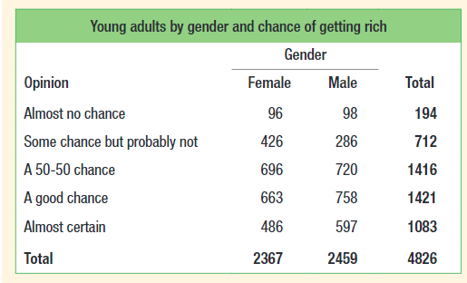
Here is an example of a two-way table:
Courtesy of Starnes, Daren S. and Tabor, Josh. The Practice of Statistics—For the AP Exam, 5th Edition. Cengage Publishing.
This table succinctly summarized a survey of 4826 people where the participants were asked about their chance of getting rich. We can see that 194 of the participants felt that they had almost no chance of getting rich and that 2367 of the participants were females. We can also see that 758 males thought that there was a good chance that they could get rich.
Joint Relative Frequencies
We can also put relative frequencies in a two-way table, where the frequencies in the table are a proportion out of the whole survey sample size. A joint relative frequency is one that has the proportion that an individual surveyed shares two characteristics, for example, being female and almost certain. The joint relative frequency for this is 486/4826 as there are 486 males who are almost certain and 4826 total people were sampled. In a joint relative frequency two-way table, the overall total in the bottom right will always be 1.00. 1️⃣
Side-by-Side Bar Graphs
Side-by-side bar graphs consist of two separate bar charts, one for each categorical variable, that are plotted next to each other. By comparing the bars in each chart, we can see how the proportions of data points in each category of one variable are related to the categories of the other variable. We can have a side-by-side bar graph where we have the joint relative frequencies for one value of one of the categorical values put side-to-side to another.
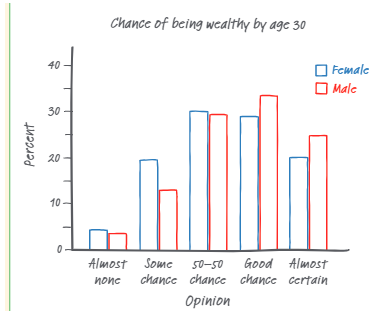
Here is an example of a side-to-side bar graph:
Courtesy of Starnes, Daren S. and Tabor, Josh. The Practice of Statistics—For the AP Exam, 5th Edition. Cengage Publishing.
Here, we have the dividing category being gender and each of the bars is the percentage of each gender who have a certain opinion about age and wealth. 💰
Segmented Bar Graphs
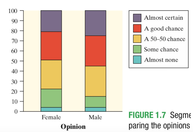
Segmented bar graphs are similar to side-by-side bar graphs, but they show the proportions of data points in each category as segments within a single bar. This can be helpful for comparing the proportions of data points within each category of one variable across the categories of the other variable. Here, the bars of each gender are stacked like this: 🍁
Courtesy of Starnes, Daren S. and Tabor, Josh. The Practice of Statistics—For the AP Exam, 5th Edition. Cengage Publishing.
In this case, we can see that the cumulative frequency for each gender is 100%. This allows us to compare the size of the different responses given by one category.
Mosaic Plots
Mosaic plots show the proportions of data points that fall into different categories by dividing the plot into rectangles that are proportional to the proportions of the data. The widths of the bars are also different, and is proportional to the number of people answering in each primary category. The areas of each of the regions relative to the whole plot are the joint relative frequencies.
Another way to think of a mosaic plot is that it is a graphic version of a two-way table. Mosaic plots can be useful for showing the relationship between two categorical variables and for comparing the proportions of data points in different categories. Here is an example of a mosaic plot:
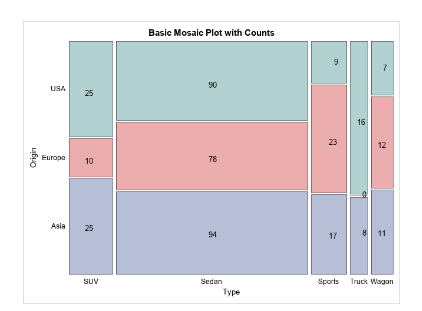
image courtesy of: blogs.sas.com
Determining Associations from Graphical Representations
In each of these, we can show if these categorical variables are associated or not. If they are associated, then we can say that they are also correlated or dependent. To do this, compare the heights (or widths) of the corresponding segments across different categories, of the heights are significantly different, then we can say that they are dependent, as this means that a certain group in one category may be more likely to have a certain response in another category but it doesn’t mean that there is a cause and effect relationship between the two. 🪢
For example, if we have data on the class level (junior, senior, etc.) and whether or not students in each class finish their homework on time, we can create a side-by-side bar graph or mosaic plot to compare the proportions of students in each class who finish their homework on time. If the proportions are significantly different across the classes, it suggests that there is an association between the two variables.
When analyzing bivariate categorical data, we can also use various methods to determine if the two variables are associated or not. If the variables are associated, it means that there is a pattern or trend in the data that suggests a relationship between the variables.
In general, it's important to keep in mind that finding an association between two variables does not necessarily mean that there is a cause-and-effect relationship between the variables. Correlation does not imply (or equal) causation. There may be other factors that are influencing the relationship between the two variables, and it is important to consider these factors when interpreting the data! 🎀
🎥 Watch: AP Stats - Exploring Two Variable Data
<< Hide Menu
2.2 Representing Two Categorical Variables
5 min read•june 18, 2024
Avanish Gupta
Jed Quiaoit
Avanish Gupta
Jed Quiaoit
Building on the stuff introduced in the previous section, there are many ways in which we can represent data from two categorical variables. Some of these are more graphical, like side-by-side bar graphs, segmented bar graphs, and mosaic plots, while others are numerical, like two-way tables (also called contingency tables). 🏟️
Various Tables and Diagrams
Two-Way Tables
Two-way tables, also known as contingency tables, consist of a table with rows and columns that correspond to the categories of the two variables. The cells of the table contain the count or percentage of data points that fall into each combination of categories. 🚦
As you can see below, two-way tables show how the individuals are distributed in the cells relative to other variables.
Here is an example of a two-way table:

Courtesy of Starnes, Daren S. and Tabor, Josh. The Practice of Statistics—For the AP Exam, 5th Edition. Cengage Publishing.
This table succinctly summarized a survey of 4826 people where the participants were asked about their chance of getting rich. We can see that 194 of the participants felt that they had almost no chance of getting rich and that 2367 of the participants were females. We can also see that 758 males thought that there was a good chance that they could get rich.
Joint Relative Frequencies
We can also put relative frequencies in a two-way table, where the frequencies in the table are a proportion out of the whole survey sample size. A joint relative frequency is one that has the proportion that an individual surveyed shares two characteristics, for example, being female and almost certain. The joint relative frequency for this is 486/4826 as there are 486 males who are almost certain and 4826 total people were sampled. In a joint relative frequency two-way table, the overall total in the bottom right will always be 1.00. 1️⃣
Side-by-Side Bar Graphs
Side-by-side bar graphs consist of two separate bar charts, one for each categorical variable, that are plotted next to each other. By comparing the bars in each chart, we can see how the proportions of data points in each category of one variable are related to the categories of the other variable. We can have a side-by-side bar graph where we have the joint relative frequencies for one value of one of the categorical values put side-to-side to another.
Here is an example of a side-to-side bar graph:

Courtesy of Starnes, Daren S. and Tabor, Josh. The Practice of Statistics—For the AP Exam, 5th Edition. Cengage Publishing.
Here, we have the dividing category being gender and each of the bars is the percentage of each gender who have a certain opinion about age and wealth. 💰
Segmented Bar Graphs
Segmented bar graphs are similar to side-by-side bar graphs, but they show the proportions of data points in each category as segments within a single bar. This can be helpful for comparing the proportions of data points within each category of one variable across the categories of the other variable. Here, the bars of each gender are stacked like this: 🍁

Courtesy of Starnes, Daren S. and Tabor, Josh. The Practice of Statistics—For the AP Exam, 5th Edition. Cengage Publishing.
In this case, we can see that the cumulative frequency for each gender is 100%. This allows us to compare the size of the different responses given by one category.
Mosaic Plots
Mosaic plots show the proportions of data points that fall into different categories by dividing the plot into rectangles that are proportional to the proportions of the data. The widths of the bars are also different, and is proportional to the number of people answering in each primary category. The areas of each of the regions relative to the whole plot are the joint relative frequencies.
Another way to think of a mosaic plot is that it is a graphic version of a two-way table. Mosaic plots can be useful for showing the relationship between two categorical variables and for comparing the proportions of data points in different categories. Here is an example of a mosaic plot:

image courtesy of: blogs.sas.com
Determining Associations from Graphical Representations
In each of these, we can show if these categorical variables are associated or not. If they are associated, then we can say that they are also correlated or dependent. To do this, compare the heights (or widths) of the corresponding segments across different categories, of the heights are significantly different, then we can say that they are dependent, as this means that a certain group in one category may be more likely to have a certain response in another category but it doesn’t mean that there is a cause and effect relationship between the two. 🪢
For example, if we have data on the class level (junior, senior, etc.) and whether or not students in each class finish their homework on time, we can create a side-by-side bar graph or mosaic plot to compare the proportions of students in each class who finish their homework on time. If the proportions are significantly different across the classes, it suggests that there is an association between the two variables.
When analyzing bivariate categorical data, we can also use various methods to determine if the two variables are associated or not. If the variables are associated, it means that there is a pattern or trend in the data that suggests a relationship between the variables.
In general, it's important to keep in mind that finding an association between two variables does not necessarily mean that there is a cause-and-effect relationship between the variables. Correlation does not imply (or equal) causation. There may be other factors that are influencing the relationship between the two variables, and it is important to consider these factors when interpreting the data! 🎀
🎥 Watch: AP Stats - Exploring Two Variable Data

© 2024 Fiveable Inc. All rights reserved.